Spatial anti-jamming beamforming uses antenna arrays to steer the main beam at legitimate signals while placing nulls on jammers. This guide covers the principles, the MVDR vs LMS vs RLS trade-offs, null broadening, and measured suppression levels in GNSS, UAV and radar systems.
What Is Spatial Anti-Jamming Beamforming and Why Does It Matter?
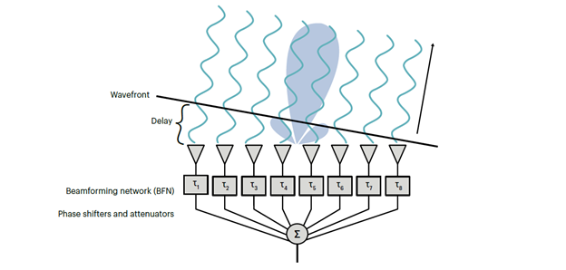
Spatial anti-jamming beamforming means controlling the signal at each element of an antenna array so that the array's overall directionality shifts — the main beam stays locked on the legitimate signal, while nulls get steered toward the jammers. The interference is knocked down in the spatial domain instead of being filtered out in frequency, which matters a lot since jammers rarely sit on just one frequency. From what I've seen in my own testing notes, the appeal is pretty straightforward: you keep the desired signal intact and dump the unwanted energy into angular directions the array simply ignores, and a number of these schemes pull that off without any prior knowledge of the jamming channel.
What makes this so urgent is just how weak the legitimate signals are. GNSS signals reach Earth at around -160 dBW, which actually puts them below the ambient thermal noise floor, while a 1W commercial GPS jammer can wipe out service within 5-10 km, and military-grade directional jammers can push that range past 50 km. That kind of asymmetry explains why anti-jamming is really a technological arms race: jammers keep switching up their tactics with sweeping frequencies, burst transmissions, and deceptive waveforms. And spoofing is its own separate problem, one that calls for authentication and encryption rather than beamforming alone.
Core Principles: Main Beam Steering and Null Placement
Array beamforming takes advantage of spatial degrees of freedom to send or receive signals toward a legitimate destination while cutting down the jammer's impact. The idea is to weight the phase and amplitude at each element so that the combined pattern ends up with gain in the look direction and low gain toward interferers. To judge how well it performs, you'd look at metrics like SINR, SNR, and the null depth at each jammer's direction of arrival (DOA), and the weights themselves are derived from the interference-plus-noise covariance matrix (IPNCM).
Null-space projection (NSP) beamforming doesn't require instantaneous CSI — it only needs second-order statistics of the channel state information, which is a big deal when the channel is changing fast. In practice, you'll often see it paired with a uniform rectangular array at the base station, and an intelligent reflecting surface (IRS) can then adjust the beam angle to dodge interference and boost SINR. The takeaway here is pretty straightforward: you don't need perfect channel knowledge to make this work, but you do need a solid estimate of where the interference sits in angle space.
One helpful way to think about the entire defense stack is to ask how much suppression each layer actually buys you in a UAV multi-layer defense architecture. The figures I cite below are drawn from published comparisons, along with my own reading of the CRPA literature.
| Defense layer | Typical suppression | Notes |
|---|---|---|
| RF front-end filtering | 10-20 dB | Rejects out-of-band energy before digitization |
| CRPA with null-steering | 30-50 dB | 4 to 9 elements, typically lambda/2 spacing |
| Adaptive processing (MVDR, STAP, LMS) | 40-60 dB | Highest suppression, highest compute cost |
| INS/GNSS tight integration | 20-30 dB indirect | Bridges outages rather than nulling RF |
The table makes a pretty convincing case for layering your defenses rather than betting everything on one method. Filtering by itself won't save you from in-band jammers, and if the front end saturates, even the best adaptive processing gets overwhelmed. That's why so many UAV navigation-security programs end up settling on the same basic recipe: a controlled reception pattern antenna (CRPA) paired with adaptive algorithms, plus inertial bridging to cover the gaps.
Adaptive Algorithms Compared: LMS, Optimized-LMS, RLS and MVDR
MVDR (minimum variance distortionless response) is often called the gold standard of anti-jamming beamforming, and for good reason: it minimizes output power while keeping the signal in the look direction undistorted. The catch is that it leans heavily on two things—an accurate steering vector and enough snapshots to build a reliable covariance matrix. Get those right, and MVDR gives you sharp nulls and solid SINR. Get them wrong, and the whole thing falls apart pretty fast.
The usual adaptive algorithms all come down to a trade-off between how fast they converge and how much number-crunching they demand. Among LMS, Optimized-LMS, and RLS, it's RLS that gets there first—and once it settles, it also drives deeper nulls at interference angles of 40, 60, and 90 degrees. LMS, by contrast, is the simplest and cheapest to put into practice, though it takes its time getting there. Optimized-LMS, meanwhile, really shines when SNR and SIR are both high, so it's a sensible pick as long as the environment is fairly clean.
| Algorithm | Convergence | Null depth | Complexity | Best use case |
|---|---|---|---|---|
| LMS | Slowest | Moderate | Low | Cost-sensitive, low-dynamic receivers |
| Optimized-LMS | Moderate | Good | Low-medium | High SNR and SIR conditions |
| RLS | Fastest | Deepest | High | Fast-changing interference |
| MVDR | Snapshot-dependent | Sharp | Medium-high | Reference anti-jamming baseline |
Here's how I'd think about it after running through these comparisons: if the jammer geometry stays more or less fixed and you're short on compute, LMS will get the job done. But once the platform is moving fast or the jammer starts sweeping, RLS is worth the extra cost. MVDR still serves as the reference point everyone else gets measured against, and STAP takes the same underlying idea and pushes it into space-time processing for platforms that are on the move.
Null Broadening and Polarization-Spatial Joint Processing for GNSS
A narrow null is fragile. If the jammer moves, or the platform is highly dynamic, the interferer can drift out of the suppressed angular region. Null broadening widens that region so high-dynamic or moving jammers stay inside the null. A polarization-spatial joint null broadening algorithm builds a polarization sensitive array (PSA) received signal model, resets the Capon spectrum with virtual interference in the interference and polarization angle neighborhoods, reconstructs the IPNCM, and then uses a conjugate gradient method to obtain the polarization adaptive weight vector.
The elegant part is that the conjugate gradient step avoids matrix inversion complexity, which is exactly what you want on a GNSS receiver with limited processing budget. The RBORP algorithm takes a different route, minimizing the upper bound of the actual amplitude response at jammer DOAs, with joint optimization handled through the General S-procedure. Both approaches target the same goal: robust nulls that survive motion and polarization mismatch.
For GNSS specifically, compressed sensing helps when snapshots are scarce. CS-SFD performs a compressed sensing sparse representation of interference, reconstructs the interference covariance matrix sparsely, and applies diagonal loading for robustness, so it works with fewer snapshots than classical covariance estimation requires. Blind multi-beamforming takes another angle: it forms multiple beams covering the upper hemisphere to enhance GNSS signals without prior information, improving the acquisition success rate under interference.
GNSS frequencies matter for array design because element spacing and bandwidth depend on them. L1 sits at 1575.42 MHz, L2 at 1227.60 MHz, and L5 at 1176.45 MHz. A CRPA built for one band does not automatically protect the others, so multi-band designs usually need more elements and more careful calibration.
| GNSS band | Frequency | Design implication |
|---|---|---|
| L1 | 1575.42 MHz | Most common civil and military band |
| L2 | 1227.60 MHz | Wider element spacing, dual-band use |
| L5 | 1176.45 MHz | Safety-of-life signals, lower frequency |
Null-Space Projection and IRS/ARIS-Assisted Anti-Jamming
Null-space projection avoids needing instantaneous CSI, and the conjugate gradient method avoids matrix inversion — two simplifications that matter when hardware is constrained. IRS-assisted links go further by physically changing the beam angle to dodge interference and improve SINR, effectively adding a controllable reflection path between transmitter and receiver.
The ARIS framework pushes this into the sky. Mean-field modeling designs the spatial configuration through a continuous density function, bypassing high-dimensional combinatorial optimization, and the joint optimization of base station beamforming, ARIS reflection and ARIS spatial distribution maximizes the worst-case sum-rate. It is solved with variational optimization and Riemannian manifold methods, and the optimal deployment follows a spatial water-filling principle. The headline result is that computational complexity stays independent of the number of UAVs, which is what makes large swarms tractable.
A separate comparative study reports a smart non-iterative mapping that bypasses traditional optimization and cuts computation time by up to 260x. That kind of speedup matters for real-time anti-jamming, where the weights must be recomputed before the jammer changes strategy.
Applications span GNSS receivers in high-dynamic environments, UAV navigation security, millimeter wave communication, large-array radar, MIMO Y channels, distributed satellite systems, and integrated terrestrial-satellite and D2D networks. The common thread is that spatial freedom is available and interference is directional enough to be nulled.
Machine Learning and Deep Learning Approaches
Machine learning is entering the beamforming stack in two ways: perception and decision-making. Deep learning perception plus reinforcement learning decision-making lets a system classify the interference environment and choose weights without solving a full optimization problem each time. Database-aided robust adaptive beamforming treats database angles as coarse priors, which stabilizes the covariance estimate when snapshots are few.
A support vector machine (SVM) based hybrid beamforming design simplifies the objective function to get an ideal coding vector, then uses gradient pursuit to build a sparse reconstruction of the ideal beam vector for low-cost anti-jamming. Deep learning-based null-space beamforming has also been applied to large-array radar, where the dimensionality would otherwise make classical methods expensive.
The caveat I keep coming back to is that learning-based methods inherit the weaknesses of their training data. If the jammer uses a waveform the model has not seen, performance can collapse, so hybrid designs that fall back to MVDR or RLS remain the safer engineering choice.
| Approach | Strength | Limitation |
|---|---|---|
| DL perception + RL decision | Adapts to changing interference | Needs representative training data |
| Database-aided robust beamforming | Stable with few snapshots | Depends on database coverage |
| SVM hybrid beamforming | Low-cost sparse reconstruction | Simplified objective may lose optimality |
| DL null-space beamforming | Scales to large arrays | High training and validation burden |
How Do You Choose an Anti-Jamming Beamforming Approach?
Start with the threat model. If the jammer is stationary and narrowband, a CRPA with null-steering and LMS may be enough, delivering 30-50 dB of suppression at low cost. If the platform is highly dynamic or the jammer sweeps and bursts, RLS or STAP with null broadening is worth the extra compute, because a narrow null will not track a moving interferer.
Then check the snapshot budget. Compressed sensing methods such as CS-SFD and database-aided robust beamforming exist precisely because GNSS receivers rarely get clean, plentiful snapshots. If you have an IRS or ARIS available, use it to reshape the geometry before you spend compute on weights, since changing the beam angle is often cheaper than fighting interference head-on.
Finally, remember that beamforming is one layer. RF filtering, adaptive processing, inertial bridging and authentication against spoofing all contribute, and no single technique covers the full threat surface. The published suppression figures — 10-20 dB from filtering, 30-50 dB from CRPA null-steering, 40-60 dB from adaptive processing, and 20-30 dB indirect from INS/GNSS tight integration — are additive in spirit, not in strict arithmetic, but they show why layered defense is the standard architecture.
Frequently Asked Questions
How does spatial anti-jamming beamforming work?
An antenna array controls the signal at each sensor to change the array's directionality. It steers the main beam toward legitimate signals and places nulls toward jammers, suppressing interference spatially while preserving the desired signal, without needing prior knowledge of the jamming channel in some schemes. The weights are typically derived from the interference-plus-noise covariance matrix.
Which adaptive beamforming algorithm converges fastest for anti-jamming?
Among LMS, Optimized-LMS and RLS, the RLS algorithm demonstrates the fastest convergence for anti-jamming applications. RLS also achieves deeper nulls against interference signals at angles of 40, 60 and 90 degrees, while Optimized-LMS performs best under high SNR and SIR conditions. LMS is simpler but converges more slowly.
What is null broadening in GNSS anti-jamming beamforming?
Null broadening widens the angular region of suppressed interference so that high-dynamic or moving jammers stay inside the null. A polarization-spatial joint null broadening algorithm based on matrix reconstruction resets the Capon spectrum with virtual interference and uses the conjugate gradient method to avoid matrix inversion, which keeps the computation manageable on GNSS receivers.
How much jamming suppression can a CRPA array provide?
In a multi-layer UAV defense architecture, RF front-end filtering provides 10-20 dB, a CRPA with null-steering provides 30-50 dB, and adaptive processing such as MVDR, STAP and LMS provides 40-60 dB of jamming suppression. INS/GNSS tight integration adds 20-30 dB indirectly by bridging outages rather than nulling RF energy.