Adaptive filtering is what keeps GNSS receivers tracking when jammers flood the band. Here is how notch filters, STAP, and CRPAs work, plus the J/S ratio and element counts that actually matter.
What Is an Anti-Jamming GNSS Receiver Adaptive Filter?
An Adaptive Filter for Anti-Jamming GNSS Receiver : a signal-processing stage follows, which as targets of its capability finds out the detractors surrounding surroundings constantly and adjusts itself to rebut these jammers in alternate ways keeping up with following satellites. It doesnt have a static filter made to the tune of one threat but retunes itself when conditions change. One practical reason it exists: GNSS satellites are in orbit about 20,000 km high; thus the signal received is weaker than background radio noise. Anything that would increase the noise floor in the GNSS band could add enough to send a receiver over its tracking threshold.
I think of anti-jam in the field as a five-part function, not just one. Continuous monitoring of signal quality and noise levels; detection of anomalous power spikes or spectral patterns; interference characterization; adaptive suppression or filtering and authentic GNSS signals preservation with tracking. Break any link and the sink either drops lock or locks on something that is not a satellite. Most of the engineering trade-offs live in this filtering stage.
How Do Adaptive Notch Filters and STAP Suppress Interference?
Adaptive notch filters (ANF) continuously estimate the instantaneous frequency of a jamming signal to filter it out from GNSS band in real time. They are the workhorse for NBI and CWI: If a jammer is on some stable frequency, just like an earthquake detector submits its reported position to monitoring stations in real time (each sampling period), so does the notch. Thus, time-domain adaptive filtering of this kind is cheap and common for fixed-band narrowband jamming suppression which explains its appearance in many front-end designs.
Space-time adaptive processing (STAP) is a GPS anti-jamming technique that rejects interference in both the spatial and temporal domains. A controlled reception pattern antenna (CRPA) employs multiple elements in a precise geometry, analyzes phase and amplitude across those elements to determine the direction of arrival, and creates spatial nulls toward the jammer while maintaining sensitivity towards satellites. When interference sources move, switch on or off the beamformer re-converges in milliseconds.
The simplest adaptive approach is least-mean-squares (LMS), which minimizes the array output power while keeping satellite gain intact. From there, you can move up to more sophisticated options like multiple-innovation filters, STAP, and compressed sensing. Interference cancellation works differently: you reconstruct the interference term and subtract it from the observations, giving you y~[n] = y[n] - i^[n]. Jamming models matter here too. When fI stays constant, you get continuous wave behavior; when fI follows a saw-tooth pattern, the result looks more chirp-like.
Time-Domain vs Space-Time Adaptive Processing: Trade-offs
Time-domain anti-jamming v/s STAP: Cost, sizing & threat geometry leads to some choices Time-domain filtering is an inexpensive method for eliminating narrowband interference, typical of fixed-band jamming. STAP incorporates spatial rejection and can filter interference compounded by physical processing from only specific directions, providing greater multi-domain suppression. The table below summarizes the comparison of both against major alternatives.
| Approach | Rejection domain | Typical strength | Main limitation |
|---|---|---|---|
| Fixed-null antenna | Spatial | Nulls one or two pre-determined directions | Cannot track new or moving threats |
| Time-domain adaptive filter | Temporal | Low cost, strong on narrowband and fixed-band jamming | No spatial discrimination |
| STAP / CRPA | Spatial and temporal | Nulls as many simultaneous threats as array degrees of freedom, tracks moving threats | Higher cost, size, and processing load |
| INS integration | None (bridging) | Carries navigation through GNSS loss for minutes to hours depending on grade | Does not remove the interference itself |
There is one trade-off that can be almost missed: a standard antenna looks around the entire sky equally, but an anti-jam antenna tries to reject lower angles (at which about every interference occurs) and instead favors higher elevation angles. That lowers the number of visible satellites, while providing up to 20 dB or more interference rejection. The other lever is frequency diversity. Some GNSSs, including GPS, broadcast on L1,L2 and L5 frequencies; so it is possible for a jammer to affect one frequency while leaving the other unaffected. As well as this dual- or multi-frequency receivers can switch over between different bands that are uneffected by jamming in order to maintain usage of location services [9]. Inertial navigation, visual odometry, barometric altimeters and terrain contour matching increase redundancy;
Key Specifications: Elements, Nulls, and J/S Ratio
The jamming-to-signal (J/S) ratio is the first number I look for in any datasheet. 70 dB J/S systems are intended for consumer jammers at short range, while 90 dB to greater than 100 dB J/S systems protect against military-grade threats. The number of elements then dictates how much you can suppress at once: A 4-element array will null 3 simultaneous jammers, a 7-element array will null six; and so forth (for this example we only consider approximations). One of the most helpful sizing rules for choosing an anti-jam antenna is that relationship between degrees of freedom and nulls.
| Specification | Safran 8230AJ | Safran 8231AJ |
|---|---|---|
| Gain | 40 dB GNSS anti-jam outdoor antenna | 40 dB GNSS anti-jam outdoor antenna |
| RF chain | Three-stage LNA, mid-section SAW, tight pre-filter | Three-stage LNA, mid-section SAW, tight pre-filter |
| Interference rejection | Adds 20 dB or more | Adds 20 dB or more |
| Dimensions | 100 mm diameter x 101.5 mm height | 100 mm diameter x 156 mm height |
| Weight | 370 g | 245 g |
| Environmental | IP67, N-type female connector, -40 to 85 C | IP67, N-type female connector, -40 to 85 C |
Those two Safran units show how much mechanical variation can hide behind nearly identical electrical specs. Same gain, same RF chain, same IP67 rating, same -40 to 85 C range — but different height and weight to fit different mounting constraints. On the receiver side, published research offers a solid performance benchmark: a time-domain adaptive filter hit the 3 dB-Hz anti-jamming target in simulations and the 8 dB-Hz target in practice, according to Song (2021, MDPI Remote Sensing 14(1):48). Keep those numbers in mind the next time a vendor claims their filter is transparent to navigation performance.
Multiplier-Free and Low-Complexity Filter Implementations
Multiplier-free implementation replaces multipliers with ROM lookup tables, distributed arithmetic, binary complement, CORDIC, multiple constant multiplication (MCM), or Canonical Signed Digit (CSD) coding. The motivation is power and area in dense digital front ends, where a wideband adaptive filter can otherwise dominate the FPGA or ASIC budget. This is also where the newest published work is most concrete.
A cascaded multiplier-free implementation reported by Song et al. (Frontiers in Physics, July 3, 2024, doi 10.3389/fphy.2024.1404236) reduces components for a 12-bit quantization anti-interference filter by one adder, 20 shift operations, and five coded word lengths compared with the traditional CSD multiplier-free technique, while keeping pseudo-range measurement deviation below 0.27 ns. That sub-nanosecond figure matters because it means the complexity savings do not come at the cost of observable ranging accuracy.
A related line of work uses nonlinear prediction rather than linear notching. A nonlinear adaptive predictor (NAP) combines a pipelined recurrent neural network (PRNN) with a tapped delay line (TDL) filter, uses gradient descent learning, and updates the linear subsection weights with normalized LMS. The appeal is that nonlinear structures can track interference that a linear notch cannot model cleanly, though they demand more careful training and validation before deployment.
Adaptive Filtering for Spoofing Detection and RFI Rejection
Adaptive filtering is not only about jamming. An adaptive antenna array provides direction-of-arrival information that forms the foundation of spoofing detection. A spoofer rebroadcasting a coherent GNSS-like signal from a single direction appears as an anomalous direction of arrival that the beamformer can flag, which is stronger evidence than relying on signal-power anomalies alone. Signal authentication and encryption, including GPS M-Code and Galileo PRS, add a cryptographic layer on top of that geometric check.
The interference types worth designing against span a wide range: wideband noise, narrowband jamming on L1 or L2, sweep jamming, proximity jamming, barrage jamming, directional jamming, and reactive jamming. Commercial products such as Septentrio AIM+, the NovAtel ITK adaptive interference suppression filter, infiniDome systems, and SBG Systems units address different slices of that list, which is why comparing them on a single number rarely works. RFI from nearby electronics is a quieter but persistent problem, and it responds well to the same adaptive notch techniques used against deliberate jammers.
Deployment Risks, Compliance, and Limitations
Jamming devices are illegal in most, though not all, countries, yet they remain easy and cheap to buy, and even simple jammers can disrupt services over several kilometers. Anti-jamming is a technological arms race: jammers use sweeping frequencies, burst transmissions, and deceptive waveforms, so a filter tuned for last year's threat may underperform against this year's. Spoofing is a distinct threat in which false satellite signals deceive receivers rather than overwhelm them, and it requires authentication and encryption rather than more filtering.
The consequences of GNSS denial are concrete and expensive: loss of drone navigation, failed autonomous missions, maritime route deviations, timing disruptions, reduced targeting accuracy, communication synchronization failures, and airspace safety concerns. For system architects, the practical conclusion is to treat adaptive filtering as one layer in a layered PNT architecture, combined with multi-frequency reception, inertial bridging, and independent timing sources, rather than as a single box that solves interference on its own.
How Do You Size an Anti-Jamming GNSS Receiver Adaptive Filter?
Start with the threat, not the hardware. Estimate the expected J/S ratio at the antenna, then pick a system with margin above it: 70 dB for consumer jammers at short range, 90 dB to 100 dB for military-grade threats. Next, count simultaneous threats and choose array elements accordingly, remembering that a 4-element array nulls 3 jammers, a 7-element array nulls 6, and a 16-element array nulls 15.
Then verify the navigation-side cost. Ask for pseudo-range measurement deviation under active filtering, the way the 2024 cascaded multiplier-free work reports deviation below 0.27 ns, and for measured anti-jamming margin in dB-Hz rather than simulation-only figures. Finally, confirm the environmental and mechanical fit: IP67 sealing, N-type female connectors, and a -40 to 85 C operating range are baseline expectations for outdoor anti-jam antennas in critical infrastructure and defense installations.
Frequently Asked Questions
How does an adaptive filter reject GNSS jamming?
Adaptive notch filters continuously estimate the instantaneous frequency of the jamming signal and dynamically filter it out of the GNSS band. Space-time adaptive processing rejects interference in both spatial and temporal domains, while array beamformers place nulls toward interference sources and preserve gain toward satellites.
What is the difference between time-domain and space-time adaptive anti-jamming?
Time-domain adaptive filtering suppresses narrowband interference at low cost and is common in fixed-band jamming scenarios. Space-time adaptive processing adds spatial rejection, handling interference from specific directions, and is widely used in GPS anti-jamming systems for stronger, multi-domain suppression.
What J/S ratio should an anti-jamming GNSS antenna handle?
The jamming-to-signal ratio is the key datasheet number. A 70 dB J/S system handles consumer jammers at short range, while 90 dB or 100 dB J/S systems address military-grade threats. Element count also matters: a 4-element array can null 3 simultaneous jammers, a 7-element array 6, and a 16-element array 15.
Can adaptive filtering also help detect GNSS spoofing?
Yes. An adaptive antenna array provides direction-of-arrival information that forms the foundation of spoofing detection. A spoofer rebroadcasting a coherent GNSS-like signal from a single direction appears as an anomalous direction of arrival that the beamformer can flag, which is stronger than relying on signal-power anomalies alone.