Direction-of-arrival estimation is the sensing layer that lets a GNSS receiver locate a jammer before it nulls it. Here is how spectral and parametric methods, sparse arrays, and CRB-driven optimization actually work in the field.
What Is GNSS Anti-Jamming DOA Estimation?
DOA estimation is what turns an antenna array into something that can actually point at a signal. In a GNSS anti-jamming chain, the order matters: first you detect that jamming is happening, then you figure out which direction the interference is coming from, and only after that can you apply a spatial filter or null to shield the receiver. Skip that angle estimate, or get it wrong, and nulling basically becomes guesswork — widen the null too much and you wipe out satellites along with the jammer, or aim it poorly and the jammer slips right through.
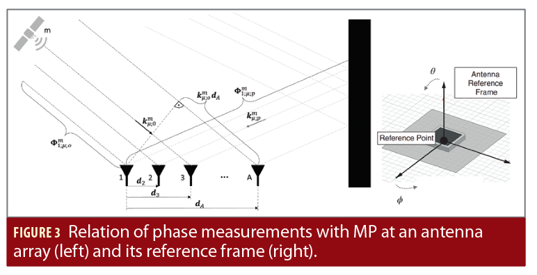
DOA is essentially a spatial estimator built on a power spectrum P(theta, phi), where the polar angle coordinates carry the real information. The binding constraint here is resolution. When two jammers sit only a few degrees apart, or a weak jammer hides near a strong satellite signal, that's where a cheap estimator quietly falls apart. Sparse arrays, the Cramér-Rao Bound, beamforming — all the other topics in this article come down to one goal: pushing that resolution limit lower.
How DOA Estimation Algorithms Work: Spectral vs Parametric
DOA methods basically fall into two camps. On one side you have spectral estimation, which works directly with the power spectrum. Take Conventional Beamforming, or the Bartlett method: it steers the array through a range of candidate angles and simply looks for peaks. Then there's Minimum Variance Distortionless Response, or MVDR, which minimizes output power while keeping a distortionless constraint in the look direction. On the other side is parametric estimation, which starts from an assumed signal model and solves for its parameters. That approach can buy you better accuracy, but it comes at a price — you're leaning much harder on your assumptions being right.
Most conventional algorithms build their cost functions around Euclidean-space distance metrics. It's a straightforward, durable approach, but it runs into a wall once you're working with only a handful of snapshots or the SNR falls apart. And that's precisely the situation GNSS jamming puts you in: the interference usually dwarfs the satellite signal, and the receiver still has to pull out a usable angle estimate in a matter of milliseconds.
The practical difference here really comes down to how the two families fail. Spectral methods tend to degrade gradually — you lose resolution, closely spaced sources start to blur together, but nothing falls off a cliff. Parametric methods, on the other hand, can pull apart sources that spectral methods would smear together, though they fall apart once the model stops matching what's actually happening in the field. From what I've seen, the decision usually has less to do with theory and more to do with how much non-nominal interference the deployment has to survive.
Sparse Arrays and Sampling for Interference Mitigation
Sparse arrays and sparse sampling are key to GNSS anti-jamming because they reduce both hardware and computational costs. Rather than filling every element of a Uniform Circular Array (UCA), a sparse non-uniform array reconfiguration picks a smaller subset of elements and works out which ones are worth keeping. The optimization problem here is quadratic fractional in form, and it's usually handled with Semi-Definite Relaxation (SDR).
A Uniform Circular Array really shines in one particular way: it can estimate DOA in both azimuth and elevation at the same time, which is a big deal when the jammer isn't conveniently sitting right on the horizon. And if you go with a sparse reconfiguration, you get to keep that same geometry while cutting down the number of channels, the front-end cost, and the size of the matrices the estimator has to invert.
Sure, the trade-off is real. When interference doesn't match the assumed model, tightly specified estimation methods lose flexibility and robustness — a limitation Inside GNSS pointed out back in 2017. Sparse designs are even more sensitive to this, since fewer elements means less redundancy to soak up model error.
Sparse arrays aren't only useful against jamming—they carry over to spoofing as well. In 2022, Y Zhao's work on coprime arrays applied the same reduced-element idea to spoofing detection, showing that the underlying principle travels across problem types. And back in 2019, M Moussa's study of GPS narrowband jammers made a similar point from a different angle: much of what makes these methods effective comes down to spatial selectivity, not simply how much raw gain you can pull from the array. Put those two together, and you get a clearer picture of why sparse designs keep showing up in anti-jam GNSS research.
Optimizing Accuracy with Cramér-Rao Bound and Spatial Correlation Coefficient
Every estimate has a theoretical floor, and the Cramér-Rao Bound (CRB) is what tells you where that floor sits. Instead of tweaking an estimator through trial and error, you treat the CRB as your objective and minimize it, which goes straight after the lowest variance the angle estimate can possibly achieve. From there, the Spatial Correlation Coefficient (SCC) comes in as a constraint to keep side-lobes in check. That way, the optimized array isn't gaining accuracy by dumping energy into directions it's supposed to reject.
Once you frame it that way, array design becomes a constrained optimization problem. Rongling LANG, Hao XU, Fei GAO, Zewen TANG, Zhipeng WANG, and Amir HUSSAIN, researchers spanning Beihang University and Edinburgh Napier University, laid out this CRB-minimization-with-SCC-constraint formulation, and they solve the resulting quadratic fractional model using Semi-Definite Relaxation.
The payoff shows up in hard conditions. A proposed algorithm achieves superior DOA estimation with fewer than 50 snapshots and an SNR below -5 dB. For anyone who has watched a receiver lose lock during a sweep jammer, those numbers are the whole point: the estimator keeps working when the signal environment is already hostile.
Compressed Sensing and Sparse Reconstruction Approaches
Compressed sensing reframes DOA estimation as a sparse recovery problem. The CS-SFD algorithm estimates the interference covariance matrix through sparse reconstruction rather than by averaging raw snapshots, then applies diagonal loading for robustness. That two-step structure is what makes it usable in practice: sparse reconstruction handles the underdetermined case, and diagonal loading keeps the inverted matrix stable when the estimate is imperfect.
The workflow is concrete. You obtain a single-shot data vector from the space-time array and vectorize it, discretize the direction space, and estimate the interference covariance matrix through sparse reconstruction. Diagonal loading is then applied before the spatial filter is computed.
I find this approach attractive precisely because it does not require dozens of clean snapshots. In a jamming scenario, the environment may change faster than a snapshot-hungry estimator can converge, so methods that work from a single vectorized observation have a structural advantage over classical covariance averaging.
Beamforming and Nulling: Bartlett and MVDR
Beamforming is where the angle estimate becomes an action. Bartlett and MVDR both produce a spatial response, but MVDR is the workhorse for anti-jamming because it places a distortionless constraint on the desired direction while minimizing total output power — effectively steering nulls toward the jammer. The quality of that null depends entirely on the accuracy of the DOA estimate feeding it.
In a representative four-channel processing chain, a four-element squared phased array feeds four coherent front-end channels. The chain identifies jamming, implements a spatial filter, and reconstructs a cleaned signal for a commercial off-the-shelf or SDR receiver. The array in that configuration uses four antennas and four in-line amplifiers, covering triple-band GPS L1/L2/L5, GLONASS G1/G2/G5, BeiDou B1/B2, and Galileo E1/E5, plus L-band correction services.
Array characterization for this kind of hardware is typically done in a spherical near-field system such as StarLab at 18 GHz, which tells you how the real array behaves before you trust a simulation.
Attitude Tracking and Multi-Satellite Fusion Under Jamming
An Attitude Reference System (ARS) aided scheme shows how far this can be pushed. It reduces 3-D attitude estimation to 1-D yaw tracking, because yaw angle variation is locally equivalent to a 1-D DOA shift. That lets the system measure yaw directly using Constrained Adaptive Monopulse (CAMP) without iterative searching.
The efficiency gain is substantial: roughly an 18x reduction in computational time compared with a highly optimized 1-D Maximum Likelihood search baseline, while maintaining high attitude accuracy with four jammers present. That work was presented at the ION 2026 Pacific PNT Meeting in Honolulu, April 13-16, 2026, pages 833-844, by Chuanrui Wang, Xiaowei Cui, Gang Liu, and Mingquan Lu.
Multi-satellite fusion based on inverse-variance weighting suppresses outliers caused by jamming or poor geometry. It is a simple idea with a large effect: measurements from satellites with degraded geometry get down-weighted automatically, so a single corrupted direction does not drag the fused solution off target.
Deployment Examples, Distortion, and Practical Limits
Deployments span rail, aviation, and defense. Cosimo Stallo and colleagues across Radiolabs, University of Roma 3, University of Rome Tor Vergata, Hitachi Rail STS, RFI, the European Space Agency, and Qascom examined GNSS anti-jamming for ERTMS train control, where the relevant metrics are probability of missed detection (Pmd) and failure rate (FR) rather than raw accuracy.
Time-domain anti-jamming (TDAJ) filters introduce a problem that array methods avoid: signal distortion and ranging bias. A preprocessing filter of optimal order can adaptively correct that distortion, but the correction itself costs complexity. Analog-domain equalization has poor accuracy and applicability, while digital-domain calibration carries high computational complexity.
Single-antenna anti-jamming sidesteps pseudo-range deviation caused by array amplitude and phase mismatch, which is genuinely advantageous for high-precision positioning. That is the honest trade-off: an array gives you spatial nulling and DOA, but it also gives you calibration burden.
The regulatory picture is uncomfortable. Jamming devices are illegal in most countries yet remain easy and cheap to buy, and simple jammers can disrupt GNSS-based services over several kilometers. Reported GNSS jamming damage has occurred in several countries, including incidents linked to North Korean activity. Related academic work includes Hong-Ki Song, Sung-Yong Lee, Seung-Hoo Lee, Jung-Beom Kim, and Changdon Kee at Seoul National University in 2012, and Xianghao Li, Zukun Lu, Feiqiang Chen, Zhe Liu, Muzi Yuan, and Gang Ou at the National University of Defense Technology in Changsha, China.
Sparse Arrays vs Full UCA: A Quick Comparison
The table below summarizes the practical trade-offs that come up most often when choosing between a full Uniform Circular Array and a sparse reconfiguration.
| Factor | Full UCA | Sparse Non-Uniform Array |
|---|---|---|
| Hardware cost | Higher: one channel per element | Lower: reduced element count |
| Computational load | Higher matrix dimensions | Reduced, solved via SDR |
| Azimuth and elevation | Concurrent estimation supported | Preserved if geometry is optimized |
| Robustness to model error | More redundancy | Less redundancy, more sensitive |
| Design objective | Coverage and gain | Minimize CRB, constrain SCC |
Sparse arrays reduce hardware and computational costs versus a full UCA, but the optimization is not free — it moves effort from silicon into design and calibration. If your interference environment is close to the assumed model, that trade is favorable. If it is not, the reduced redundancy becomes a liability, and a full array with more elements may be the more forgiving choice.
How Does GNSS Anti-Jamming DOA Estimation Work in Practice?
In practice the chain runs in a fixed order. Jamming detection comes first, then DOA estimation of the jamming signal, then a spatial filter or null that minimizes jammer impact and cleans the useful signal before it reaches the GNSS receiver. Each stage depends on the one before it, which is why detection latency and estimation resolution both matter.
The four-channel example ties it together: identify jamming, apply the spatial filter, reconstruct the signal, and hand it to a COTS or SDR receiver. The receiver firmware algorithms then apply digital filters to detect and remove residual jamming before the positioning engine ever sees the data.
That layering is deliberate. Array processing handles the spatial dimension, firmware handles what leaks through, and the positioning engine is protected from both. When the layers are designed together, a receiver can keep producing a fix while a jammer is still transmitting.
Spectral vs Parametric Estimation at a Glance
The comparison below is the one I use when explaining the two families to engineers who are new to the topic.
| Attribute | Spectral Estimation | Parametric Estimation |
|---|---|---|
| Basis | Power spectrum | Model-based parameters |
| Examples | Bartlett, MVDR | Model-fitting estimators |
| Few snapshots | Degrades | Can still resolve |
| Model mismatch | Graceful degradation | Can fail sharply |
| Typical use | Real-time nulling | High-resolution analysis |
Spectral estimation uses the power spectrum; parametric estimation uses model-based parameters. Neither dominates. For real-time nulling on a moving platform, the spectral family is usually the safer bet because its failure mode is gradual. For offline analysis or tightly controlled geometry, parametric methods extract more resolution from the same data.
Frequently Asked Questions
How does DOA estimation support GNSS anti-jamming?
Jamming detection is the first step in mitigation. The system estimates the jammer's direction of arrival using antenna array processing, then applies a spatial filter or nulling to minimize jammer impact, cleaning the useful signal before it reaches the GNSS receiver. Without an accurate angle, nulling either misses the jammer or suppresses legitimate satellite signals.
What are the main categories of DOA estimation methods?
Methods for estimating a jamming signal's DOA are largely classified two ways: spectral estimation and parametric estimation. Beamforming and nulling approaches such as Conventional Beamforming (Bartlett) and Minimum Variance Distortionless Response (MVDR) fall under spectral estimation. Parametric methods instead assume a signal model and solve for its parameters, trading robustness for higher resolution.
Why use sparse arrays for GNSS interference DOA estimation?
Sparse arrays and sparse sampling reduce hardware and computational costs. A reduced number of array elements can be selected to reconstruct a non-uniform sparse array from a Uniform Circular Array, lowering complexity while maintaining DOA estimation accuracy and robustness. The reconfiguration is a quadratic fractional optimization typically solved by Semi-Definite Relaxation, with the Cramér-Rao Bound minimized and side-lobes constrained.
What role does the Cramér-Rao Bound play in DOA estimation?
Minimizing the Cramér-Rao Bound (CRB) is used as the objective to ensure DOA estimation accuracy. The Spatial Correlation Coefficient (SCC) is added as a constraint to mitigate side-lobes, and the resulting quadratic fractional model is solved by Semi-Definite Relaxation (SDR). This approach has demonstrated superior estimation with fewer than 50 snapshots and SNR below -5 dB.